Wolfram Mathematica How to Make X Become X Again

• WolframAlpha.com
• WolframCloud.com
• All Sites & Public Resources...

TECH Note

Manipulating Equations and Inequalities

"Defining Variables" discussed assignments such equally x=y , which set ten equal to y . Here we talk over equations, which test equality. The equation x==y tests whether x is equal to y .

This tests whether 2+2 and 4 are equal. The issue is the symbol True:

It is very important that you practise not confuse x=y with x==y . While ten=y is an imperative statement that actually causes an assignment to be washed, 10==y but tests whether ten and y are equal, and causes no explicit action. If y'all accept used the C programming linguistic communication, you volition recognize that the notation for assignment and testing in the Wolfram Language is the same as in C.

x=y	assigns 10 to have value y
ten==y	tests whether x and y are equal

This assigns x to accept value 4:

If you enquire for x, you lot now get 4:

This tests whether x is equal to 4. In this case, it is:

This removes the value assigned to 10:

The tests used then far involve only numbers, and always give a definite answer, either True or False. You can besides exercise tests on symbolic expressions.

The Wolfram Language cannot get a definite event for this test unless y'all give ten a specific numerical value:

If you lot replace ten by the specific numerical value four, the test gives False:

Even when you practice tests on symbolic expressions, there are some cases where you tin get definite results. An important 1 is when y'all test the equality of ii expressions that are identical. Whatever the numerical values of the variables in these expressions may be, the Wolfram Language knows that the expressions must ever exist equal.

The two expressions are identical, and so the result is Truthful, any the value of x may exist:

The Wolfram Language does not try to tell whether these expressions are equal. In this case, using Expand would make them take the same grade:

Expressions like x==4 represent equations in the Wolfram Language. There are many functions in the Wolfram Language for manipulating and solving equations.

This is an equation in the Wolfram Language. "Solving Equations" discusses how to solve it for ten:

You tin can assign a name to the equation:

If you lot ask for eqn, you now get the equation:

An expression like x^ii+2x-7==0 represents an equation in the Wolfram Language. You will often need to solve equations similar this, to discover out for what values of x they are true.

This gives the ii solutions to the quadratic equation 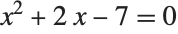. The solutions are given as replacements for 10:

Hither are the numerical values of the solutions:

You can get a listing of the bodily solutions for x by applying the rules generated by Solve to x using the replacement operator:

You can equally well utilize the rules to any other expression involving x:

Solve[ lhs==rhs , x ]	solve an equation, giving a list of rules for x
x/.solution	utilise the list of rules to go values for x
expr/.solution	use the list of rules to get values for an expression

Finding and using solutions to equations.

Solve always tries to give you explicit formulas for the solutions to equations. However, it is a basic mathematical result that, for sufficiently complicated equations, explicit algebraic formulas in terms of radicals cannot be given. If you accept an algebraic equation in one variable, and the highest power of the variable is at most four, then the Wolfram Language can always give you lot formulas for the solutions. Even so, if the highest power is five or more, it may be mathematically incommunicable to give explicit algebraic formulas for all the solutions.

The Wolfram Language can e'er solve algebraic equations in 1 variable when the highest power is less than 5:

It can solve some equations that involve higher powers:

There are some equations, however, for which it is mathematically impossible to find explicit formulas for the solutions. The Wolfram Language uses Root objects to correspond the solutions in this example:

Even though you cannot get explicit formulas, you can still evaluate the solutions numerically:

In addition to being able to solve purely algebraic equations, the Wolfram Linguistic communication can also solve some equations involving other functions.

Here the Wolfram Language returns a complete solution to the equation:

Here, subsequently printing a warning, the Wolfram Language returns one solution to the equation:

Information technology is important to realize that an equation such as actually has an space number of possible solutions. However, Solve past default returns just one solution, only prints a message telling you lot that other solutions may exist. Y'all tin utilize Reduce to go more information.

In that location is no explicit "airtight class" solution for a transcendental equation like this:

You can find an approximate numerical solution using FindRoot and giving a starting value for x:

Solve tin also handle equations involving symbolic functions. In such cases, it again prints a alarm, then gives results in terms of formal changed functions.

The Wolfram Language returns a consequence in terms of the formal inverse function of f:

Solve[ { lhs 1 ==rhs 1 , lhs 2 ==rhs two , … } , { x , y , … } ]
	solve a gear up of simultaneous equations for 10 , y , …

Solving sets of simultaneous equations.

You tin can also utilize the Wolfram Language to solve sets of simultaneous equations. You just give the list of equations and specify the list of variables to solve for.

Hither is a list of two simultaneous equations, to be solved for the variables x and y:

Here are some more complicated simultaneous equations. The two solutions are given every bit two lists of replacements for x and y:

This uses the solutions to evaluate the expression x+y:

The Wolfram Language can solve any set of simultaneous linear or polynomial equations.

When you are working with sets of equations in several variables, it is often user-friendly to reorganize the equations by eliminating some variables betwixt them.

This eliminates y betwixt the ii equations, giving a single equation for 10:

If you take several equations, there is no guarantee that there exists any consistent solution for a particular variable.

There is no consistent solution to these equations, so the Wolfram Language returns { } , indicating that the set of solutions is empty:

There is also no consistent solution to these equations for most all values of a:

The general question of whether a prepare of equations has any consistent solution is quite a subtle one. For example, for most values of a, the equations {x==1,x==a} are inconsistent, so at that place is no possible solution for 10. All the same, if a is equal to ane, then the equations do accept a solution. Solve is gear up up to requite you generic solutions to equations. It discards whatsoever solutions that exist merely when special constraints between parameters are satisfied.

If you apply Reduce instead of Solve, the Wolfram Language will, however, keep all the possible solutions to a set up of equations, including those that require special conditions on parameters.

This shows that the equations have a solution but when a==1. The note a==1&&x==1 represents the requirement that both a==1 and ten==i should be True:

This gives the complete set of possible solutions to the equation. The reply is stated in terms of a combination of simpler equations. && indicates equations that must simultaneously be true; | | indicates alternatives:

This gives a more than complicated combination of equations:

This gives a symbolic representation of all solutions:

Solve[ lhs==rhs , ten ]	solve an equation for x
Solve[ { lhs one ==rhs 1 , lhs 2 ==rhs ii , … } , { x , y , … } ]
	solve a set of simultaneous equations for ten , y , …
Eliminate[ { lhs 1 ==rhs 1 , lhs 2 ==rhs ii , … } , { x , … } ]
	eliminate x , … in a prepare of simultaneous equations
Reduce[ { lhs 1 ==rhs 1 , lhs ii ==rhs 2 , … } , { x , y , … } ]
	give a set up of simplified equations, including all possible solutions

Functions for solving and manipulating equations.

Reduce also has powerful capabilities for treatment equations specifically over real numbers or integers. "Equations and Inequalities over Domains" discusses this in more detail.

This reduces the equation assuming x and y are complex:

This includes the conditions for x and y to exist real:

This gives only the integer solutions:

The Representation of Equations and Solutions

The Wolfram Organisation treats equations as logical statements. If you type in an equation like x^ii+3x==ii, the Wolfram System interprets this equally a logical statement that asserts that x^two+3x is equal to 2. If you have assigned an explicit value to x, say ten=four, then the Wolfram System can explicitly decide that the logical statement ten^ii+3x==2 is Fake.

If you accept not assigned any explicit value to 10, however, the Wolfram System cannot work out whether x^2+3x==2 is Truthful or False. Every bit a consequence, it leaves the equation in the symbolic form x^2+3x==2.

You tin dispense symbolic equations in the Wolfram System in many ways. I common goal is to rearrange the equations so as to "solve" for a item set of variables.

Here is a symbolic equation:

You can use the role Reduce to reduce the equation so equally to give "solutions" for 10. The result, similar the original equation, can be viewed as a logical statement:

The quadratic equation x^2+3x==2 tin can exist thought of every bit an implicit argument nearly the value of x. Every bit shown in the previous example, you tin can apply the part Reduce to get a more explicit statement most the value of x. The expression produced by Reduce has the course 10==r ₁ | | 10==r _two . This expression is again a logical argument, which asserts that either x is equal to r _one , or x is equal to r ₂ . The values of x that are consistent with this statement are exactly the same every bit the ones that are consistent with the original quadratic equation. For many purposes, however, the class that Reduce gives is much more useful than the original equation.

You tin combine and manipulate equations just like other logical statements. You tin can use logical connectives such equally | | and && to specify culling or simultaneous conditions. You tin can use functions like LogicalExpand, every bit well as FullSimplify, to simplify collections of equations.

For many purposes, you will notice it convenient to manipulate equations simply as logical statements. Sometimes, yet, yous will actually want to utilize explicit solutions to equations in other calculations. In such cases, it is convenient to convert equations that are stated in the form lhs==rhs into transformation rules of the form lhs rhs. Once you accept the solutions to an equation in the form of explicit transformation rules, you lot can substitute the solutions into expressions by using the /. operator.

Reduce produces a logical statement about the values of x corresponding to the roots of the quadratic equation:

ToRules converts the logical statement into an explicit list of transformation rules:

You tin can now use the transformation rules to substitute the solutions for x into expressions involving x:

The function Solve produces transformation rules for solutions directly:

Equations in One Variable

The main equations that Solve and related Wolfram Linguistic communication functions deal with are polynomial equations.

It is easy to solve a linear equation in x:

I can also solve quadratic equations just by applying a simple formula:

The Wolfram Language can also find exact solutions to cubic equations. Here is the showtime solution to a insufficiently simple cubic equation:

For cubic and quartic equations, the results are often complicated, only for all equations with degrees upwardly to iv the Wolfram Language is ever able to give explicit formulas for the solutions.

An important feature of these formulas is that they involve only radicals: arithmetics combinations of foursquare roots, cube roots and college roots.

Information technology is a fundamental mathematical fact, still, that for equations of caste 5 or college, it is no longer possible in full general to give explicit formulas for solutions in terms of radicals.

There are some specific equations for which this is still possible, only in the vast majority of cases it is not.

This constructs a degree-six polynomial:

For a polynomial that factors in the way this one does, information technology is straightforward for Solve to detect the roots:

This constructs a polynomial of degree eight:

The polynomial does not factor, merely it can exist decomposed into nested polynomials, and so Solve can over again find explicit formulas for the roots:

Root[ f , g ]

the k th root of the equation f [ x ] ==0

Implicit representation for roots.

No explicit formulas for the solution to this equation can be given in terms of radicals, so the Wolfram Language uses an implicit symbolic representation:

This finds a numerical approximation to each root:

If what you desire in the end is a numerical solution, it is usually much faster to employ NSolve from the outset:

Root objects provide an exact, though implicit, representation for the roots of a polynomial. You tin work with them much equally you lot would work with Sqrt[2] or any other expression that represents an exact numerical quantity.

Here is the Root object representing the first root of the polynomial discussed previously:

This is a numerical approximation to its value:

Round does an exact computation to discover the closest integer to the root:

If you substitute the root into the original polynomial, and then simplify the outcome, you lot get zero:

This finds the product of all the roots of the original polynomial:

The complex conjugate of the third root is the second root:

If the just symbolic parameter that exists in an equation is the variable that y'all are solving for, then all the solutions to the equation volition merely be numbers. But if there are other symbolic parameters in the equation, then the solutions will typically be functions of these parameters.

The solution to this equation tin once more be represented by Root objects, only now each Root object involves the parameter a:

When a is replaced with ane, the Root objects can exist simplified, and some are given as explicit radicals:

This shows the behavior of the offset root every bit a function of a:

This finds the derivative of the commencement root with respect to a:

Solve gives two identical solutions to this equation:

Here are the first 4 solutions to a 10 ^th-degree equation. The solutions come in pairs:

The Wolfram Language also knows how to solve equations that are non explicitly in the class of polynomials.

Here is an equation involving foursquare roots:

And here is i involving logarithms:

So long as it can reduce an equation to some kind of polynomial form, the Wolfram Language will always be able to represent its solution in terms of Root objects. However, with more full general equations, involving, say, transcendental functions, there is no systematic mode to apply Root objects, or even necessarily to observe numerical approximations.

Hither is a simple transcendental equation for x:

In that location is no solution to this equation in terms of standard functions:

The Wolfram Language can nonetheless detect a numerical solution even in this example:

Polynomial equations in one variable only ever have a finite number of solutions. But transcendental equations frequently take an infinite number. Typically the reason for this is that transcendental functions in effect have infinitely many possible inverses. With the default option setting InverseFunctionsTrue, Solve will notwithstanding assume that there is a definite inverse for whatsoever such function. Solve may then be able to return particular solutions in terms of this changed function.

The Wolfram Linguistic communication returns a particular solution in terms of ProductLog, but prints a warning indicating that other solutions may be lost:

If yous enquire Solve to solve an equation involving an arbitrary function like f, it volition by default try to construct a formal solution in terms of changed functions.

Solve by default uses a formal changed for the function f:

This is the structure of the inverse function:

This returns an explicit inverse role:

The Wolfram Language can practise formal operations on inverse functions:

While Solve can only requite specific solutions to an equation, Reduce can give a representation of a whole solution set. For transcendental equations, information technology ofttimes ends up introducing new parameters, say with values ranging over all possible integers.

This is a complete representation of the solution gear up:

Here over again is a representation of the general solution:

Every bit discussed at more length in "Equations and Inequalities over Domains", Reduce allows y'all to restrict the domains of variables. Sometimes this will let yous generate definite solutions to transcendental equations—or testify that they do not exist.

With the domain of 10 restricted, this yields definite solutions:

With ten constrained to be real, only one solution is possible:

Reduce knows there tin exist no solution here:

Counting and Isolating Polynomial Roots

Counting Roots of Polynomials

CountRoots[ poly , x ]	requite the number of real roots of the polynomial poly in x
CountRoots[ poly , { x , a , b } ]	give the number of roots of the polynomial poly in x with

Counting roots of polynomials.

CountRoots accepts polynomials with Gaussian rational coefficients. The root count includes multiplicities.

This gives the number of real roots of :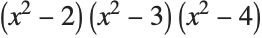

This counts 17 ^th-degree roots of unity in the closed unit square:

The coefficients of the polynomial can exist Gaussian rationals:

Isolating Intervals

RootIntervals[ { poly 1 , poly 2 , … } ]	give a listing of disjoint isolating intervals for the real roots of any of the poly i , together with a listing of which polynomials really have each successive root
RootIntervals[ poly ]	give disjoint isolating intervals for real roots of a single polynomial
RootIntervals[ polys ,Complexes]	requite disjoint isolating intervals or rectangles for circuitous roots of polys
IsolatingInterval[ a ]	give an isolating interval for the algebraic number a
IsolatingInterval[ a , dx ]	give an isolating interval of width at near dx

Functions for isolating roots of polynomials.

RootIntervals accepts polynomials with rational number coefficients.

Here are isolating intervals for the real roots of :

The 2d listing shows which interval contains a root of which polynomial:

This gives isolating intervals for all complex roots of :

Hither are isolating intervals for the 3rd- and quaternary-degree roots of unity. The 2nd interval contains a root common to both polynomials:

Here is an isolating interval for a root of a polynomial of degree 7:

This gives an isolating interval of width at most :

All numbers in the interval have the first 10 decimal digits in common:

Root[ f , k ]

the k thursday root of the polynomial equation f [ x ] ==0

The representation of algebraic numbers.

When you enter a Root object, the polynomial that appears in it is automatically reduced to a minimal course:

This extracts the pure function that represents the polynomial, and applies it to x:

Root objects are the manner that the Wolfram Linguistic communication represents algebraic numbers. Algebraic numbers have the property that when you perform algebraic operations on them, you ever go a single algebraic number as the consequence.

Here is the square root of an algebraic number:

Here is a more complicated expression involving an algebraic number:

Again this can be reduced to a single Root object, albeit a fairly complicated ane:

Operations on algebraic numbers.

In this uncomplicated case, the Root object is automatically expressed in terms of radicals:

When cubic polynomials are involved, Root objects are not automatically expressed in terms of radicals:

This gives a Root object involving a degree-vi polynomial:

Even though a simple class in terms of radicals does exist, ToRadicals does not detect it:

Beyond degree four, most polynomials do not take roots that can be expressed at all in terms of radicals. Even so, for caste five it turns out that the roots can always be expressed in terms of elliptic or hypergeometric functions. The results, however, are typically much also complicated to be useful in practice.

RootSum[ f , form ]	the sum of form [ 10 ] for all satisfying the polynomial equation f [ ten ] ==0
Normal[ expr ]	the form of expr with RootSum replaced past explicit sums of Root objects

This computes the sum of the reciprocals of the roots of :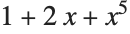

At present no explicit result tin can exist given in terms of radicals:

This expands the RootSum into an explicit sum involving Root objects:

RootApproximant[ x ]	converts the number x to i of the "simplest" algebraic numbers that approximates it well
RootApproximant[ x , n ]	finds an algebraic number of degree at most due north that approximates x

This recovers from a numerical approximation:

In this case, the result has caste at virtually 4:

This confirms that the Root expression does represent to :

You can requite Solve a list of simultaneous equations to solve. Solve tin find explicit solutions for a large class of simultaneous polynomial equations.

Hither is a simple linear equation with 2 unknowns:

Here is a more than complicated example. The effect is a listing of solutions, with each solution consisting of a list of transformation rules for the variables:

You can use the listing of solutions with the /. operator:

Even when Solve cannot find explicit solutions, it frequently tin "unwind" simultaneous equations to produce a symbolic result in terms of Root objects:

Yous tin can then use North to go a numerical event:

The variables that you employ in Solve do not need to be single symbols. Oftentimes when you prepare large collections of simultaneous equations, you lot will want to use expressions similar a [ i ] as variables.

Hither is a list of three equations for the a[i]:

This solves for some of the a[i]:

Solve[ eqns , { x 1 , x 2 , … } ]	solve eqns for the specific objects ten i
Solve[ eqns ]	try to solve eqns for all the objects that appear in them

Solving simultaneous equations.

If you do non explicitly specify objects to solve for, Solve will try to solve for all the variables:

■ Solve[ { lhs 1 ==rhs one , lhs 2 ==rhs two , … } , vars ]

■ Solve[ lhs i ==rhs ane &&lhs ii ==rhs 2 && … , vars ]

■ Solve[ { lhs ane , lhs two , … }=={ rhs 1 , rhs 2 , … } , vars ]

Ways to present simultaneous equations to Solve.

If you lot construct simultaneous equations from matrices, y'all typically become equations between lists of expressions:

Solve converts equations involving lists to lists of equations:

In some kinds of computations, it is convenient to work with arrays of coefficients instead of explicit equations. Y'all can construct such arrays from equations by using CoefficientArrays.

Generic and Non‐Generic Solutions

If you have an equation similar 2x==0, it is perfectly articulate that the only possible solution is x0. However, if you accept an equation like ax==0, things are not and then clear. If a is not equal to cypher, then x0 is over again the only solution. However, if a is in fact equal to zero, and so whatsoever value of x is a solution. You tin can see this past using Reduce.

Solve implicitly assumes that the parameter a does not accept the special value 0:

Reduce, on the other hand, gives yous all the possibilities, without bold annihilation virtually the value of a:

A basic difference between Reduce and Solve is that Reduce gives all the possible solutions to a set of equations, while Solve gives only the generic ones. Solutions are considered "generic" if they involve conditions simply on the variables that you explicitly solve for, and not on other parameters in the equations. Reduce and Solve also differ in that Reduce always returns combinations of equations, while Solve gives results in the form of transformation rules.

Solve[ eqns , vars ]	find generic solutions to equations
Reduce[ eqns , vars ]	reduce equations, maintaining all solutions

This is the solution to an arbitrary linear equation given by Solve:

Reduce gives the full version, which includes the possibility a==b==0. In reading the output, note that && has college precedence than | | :

Hither is the full solution to a full general quadratic equation. At that place are three alternatives. If a is nonzero, and then there are two solutions for ten, given by the standard quadratic formula. If a is aught, even so, the equation reduces to a linear one. Finally, if a, b and c are all zero, at that place is no restriction on ten:

When you accept several simultaneous equations, Reduce can show you under what conditions the equations have solutions. Solve shows you whether there are any generic solutions.

This shows in that location can never exist any solution to these equations:

At that place is a solution to these equations, but only when a has the special value 1:

The solution is not generic, and is rejected by Solve:

But if a is constrained to take value 1, then Solve once again returns a solution:

This equation is true for whatever value of 10:

This is the kind of result Solve returns when yous give an equation that is always true:

When yous piece of work with systems of linear equations, you lot can utilise Solve to go generic solutions and Reduce to find out for what values of parameters solutions be.

The matrix has determinant zip:

This makes a set of three simultaneous equations:

Solve reports that there are no generic solutions:

Reduce, however, shows that in that location would be a solution if the parameters satisfied the special status a==2b-c:

For nonlinear equations, the weather condition for the existence of solutions can be much more complicated.

Here is a very simple pair of nonlinear equations:

Solve shows that the equations have no generic solutions:

Reduce gives the consummate conditions for a solution to exist:

When you write down a prepare of simultaneous equations in the Wolfram Language, you lot are specifying a collection of constraints between variables. When you utilize Solve, you lot are finding values for some of the variables in terms of others, subject to the constraints represented past the equations.

Solve[ eqns , vars , elims ]	find solutions for vars , eliminating the variables elims
Eliminate[ eqns , elims ]	rearrange equations to eliminate the variables elims

Hither are two equations involving x, y and the "parameters" a and b:

If you solve for both x and y, you go results in terms of a and b:

Similarly, if y'all solve for 10 and a, you lot become results in terms of y and b:

If you simply want to solve for x, withal, yous have to specify whether yous want to eliminate y or a or b. This eliminates y, then gives the outcome in terms of a and b:

If you lot eliminate a, then you get a result in terms of y and b:

In some cases, you may want to construct explicitly equations in which variables have been eliminated. You lot can practise this using Eliminate.

This combines the two equations in the listing eqn by eliminating the variable a:

This is what you lot get if you eliminate y instead of a:

To solve the problem, simply write f in terms of a and b, eliminating the original variables 10 and y:

In dealing with sets of equations, it is mutual to consider some of the objects that appear equally truthful "variables", and others equally "parameters". In some cases, y'all may demand to know for what values of parameters a particular relation between the variables is always satisfied.

SolveAlways[ eqns , vars ]

solve for the values of parameters for which the eqns are satisfied for all values of the vars

Solving for parameters that brand relations always truthful.

This finds the values of parameters that brand the equation hold for all x:

This finds values of the undetermined coefficients:

Relational and Logical Operators

x==y	equal (besides input as 10  y )
x!=y	unequal (too input as 10 ≠ y )
x>y	greater than
x>=y	greater than or equal to (too input as x ≥ y )
10<y	less than
ten<=y	less than or equal to (as well input as 10 ≤ y )
x==y==z	all equal
x!=y!=z	all diff (singled-out)
x>y>z , etc.	strictly decreasing, etc.

This tests whether x is less than 7. The issue is Imitation:

Non all of these numbers are unequal, so this gives False:

Since both of the quantities involved are numeric, the Wolfram Linguistic communication can determine that this is true:

The Wolfram Language does not know whether this is true or false:

!p	not (likewise input equally ¬ p )
p&&q&& …	and (also input every bit p ∧ q ∧ … )
p | | q | | …	or (as well input as p ∨ q ∨ … )
Xor[ p , q , … ]	sectional or (besides input as p ⊻ q ⊻ … )
Nand[ p , q , … ] and Nor[ p , q , … ]	nand and nor (also input as ⊼ and ⊽ )
If[ p , then , else ]	give so if p is True , and else if p is Faux
LogicalExpand[ expr ]	expand out logical expressions

Both tests give True, then the result is Truthful:

You should call up that the logical operations ==, && and | | are all double characters in the Wolfram Language. If you lot take used a programming language such as C, you lot will exist familiar with this notation.

The Wolfram Language does not know whether this is true or false:

The Wolfram Linguistic communication leaves this expression unchanged:

Solving Logical Combinations of Equations

When you give a list of equations to Solve, information technology assumes that you want all the equations to be satisfied simultaneously. It is also possible to give Solve more complicated logical combinations of equations.

Solve assumes that the equations ten+y==ane and x-y==2 are simultaneously valid:

Here is an alternative grade, using the logical connective && explicitly:

This specifies that either x+y==i or 10-y==two. Solve gives two solutions for x, corresponding to these two possibilities:

Solve gives three solutions to this equation:

If yous explicitly include the exclamation that x!=0, one of the previous solutions is suppressed:

Here is a slightly more complicated example. Note that the precedence of | | is lower than the precedence of &&, so the equation is interpreted equally (x^3==x&&x!=ane) | |x^ii==two , not 10^3==10&&(x!=ane| |ten^2==2) :

When you use Solve, the final results yous get are in the grade of transformation rules. If you lot use Reduce or Eliminate, on the other paw, so your results are logical statements, which you can dispense further.

This gives a logical argument representing the solutions of the equation 10^2==x:

This finds values of ten that satisfy x^v==ten merely practise not satisfy the statement representing the solutions of x^ii==x:

The logical statements produced by Reduce tin be thought of as representations of the solution prepare for your equations. The logical connectives &&, | | and and then on then correspond to operations on these sets.

eqns 1 | | eqns 2	union of solution sets
eqns 1 &&eqns 2	intersection of solution sets
!eqns	complement of a solution set
Implies[ eqns i , eqns 2 ]	the part of eqns 1 that contains eqns 2

Operations on solution sets.

You lot may often find it convenient to use special notations for logical connectives, as discussed in "Operators".

The input uses special notations for Implies and Or:

Merely as the equation x^2+3x==2 asserts that x^2+3x is equal to two, then besides the inequality 10^2+3x>ii asserts that x^2+3x is greater than ii. In the Wolfram Linguistic communication, Reduce works not just on equations, simply also on inequalities.

Reduce[ { ineq i , ineq 2 , … } , ten ]

reduce a collection of inequalities in ten

Manipulating univariate inequalities.

This pair of inequalities reduces to a unmarried inequality:

These inequalities can never simultaneously be satisfied:

When practical to an equation, Reduce[ eqn , x ] tries to get a result consisting of simple equations for ten of the form 10==r _one , …. When applied to an inequality, Reduce[ ineq , x ] does the exactly coordinating thing, and tries to get a result consisting of uncomplicated inequalities for x of the form l ₁ <x<r ₁ , ….

This reduces a quadratic equation to 2 uncomplicated equations for x:

This reduces a quadratic inequality to 2 simple inequalities for x:

This inequality yields three distinct intervals:

The ends of the intervals are at roots and poles:

Solving this inequality requires introducing ProductLog:

Transcendental functions like have graphs that get up and down infinitely many times, so that infinitely many intervals tin can exist generated.

The 2d inequality allows only finitely many intervals:

This is how Reduce represents infinitely many intervals:

Fairly unproblematic inputs tin give fairly complicated results:

If you accept inequalities that involve <= as well equally <, there may be isolated points where the inequalities can be satisfied. Reduce represents such points past giving equations.

This inequality can be satisfied at just two isolated points:

This yields both intervals and isolated points:

Reduce[ { ineq i , ineq ii , … } , { 10 i , x 2 , … } ]

reduce a collection of inequalities in several variables

Multivariate inequalities.

For inequalities involving several variables, Reduce in outcome yields nested collections of interval specifications, in which subsequently variables have bounds that depend on earlier variables.

This represents the unit disk as nested inequalities for x and y:

In geometrical terms, any linear inequality divides space into ii halves. Lists of linear inequalities thus ascertain polyhedra, sometimes bounded, sometimes non. Reduce represents such polyhedra in terms of nested inequalities. The corners of the polyhedra e'er appear among the endpoints of these inequalities.

This defines a triangular region in the aeroplane:

Even a single triangle may demand to be described as two components:

Lists of inequalities in general stand for regions of overlap betwixt geometrical objects. Often the description of these can be quite complicated.

This represents the part of the unit disk on one side of a line:

Here is the intersection between ii disks:

If the disks are as well far apart, in that location is no intersection:

Here is an example involving a transcendental inequality:

If you accept inequalities that involve parameters, Reduce automatically handles the different cases that tin occur, but equally it does for equations.

The form of the intervals depends on the value of a:

One gets a hyperbolic or an elliptical region, depending on the value of a:

Reduce tries to requite you lot a complete description of the region defined past a set of inequalities. Sometimes, however, you may just want to find private instances of values of variables that satisfy the inequalities. You tin can practice this using FindInstance.

FindInstance[ ineqs , { ten 1 , x 2 , … } ]	try to discover an instance of the x i satisfying ineqs
FindInstance[ ineqs , vars , due north ]	try to observe n instances

Finding private points that satisfy inequalities.

This finds a specific example that satisfies the inequalities:

This shows that at that place is no way to satisfy the inequalities:

FindInstance is in some ways an analog for inequalities of Solve for equations. Similar Solve, information technology returns a list of rules giving specific values for variables. Only while for equations these values tin generically give an authentic representation of all solutions, for inequalities they can simply stand for to isolated sample points within the regions described by the inequalities.

Every time you call FindInstance with specific input, it volition give the same output. And when there are instances that stand for to special, limiting points of some kind, information technology will preferentially return these. But in full general, the distribution of instances returned by FindInstance will typically seem somewhat random. Each instance is, even so, in effect a constructive proof that the inequalities you have given tin can in fact be satisfied.

If y'all ask for i betoken in the unit disk, FindInstance gives the origin:

This finds 500 points in the unit disk:

Their distribution seems somewhat random:

Equations and Inequalities over Domains

The Wolfram Language ordinarily assumes that variables that appear in equations can represent arbitrary complex numbers. Simply when yous employ Reduce, you can explicitly tell the Wolfram Language that the variables correspond objects in more restricted domains.

Reduce by default assumes that x can be complex, and gives all v circuitous solutions:

But hither it assumes that x is existent, and gives simply the existent solutions:

And here it assumes that ten is an integer, and gives only the integer solutions:

A single polynomial equation in i variable will always take a finite set of discrete solutions. And in such a case, 1 can retrieve of Reduce[ eqns , vars , dom ] as only filtering the solutions by selecting the ones that happen to lie in the domain dom .

Just as before long equally there are more variables, things can go more complicated, with solutions to equations corresponding to parametric curves or surfaces in which the values of some variables tin can depend on the values of others. Oftentimes this dependence can be described by some collection of equations or inequalities, simply the form of these can alter significantly when one goes from 1 domain to some other.

This gives solutions over the circuitous numbers every bit simple formulas:

To stand for solutions over the reals requires introducing an inequality:

Over the integers, the solution can be represented every bit equations for discrete points:

If your input involves only equations, so Reduce volition by default assume that all variables are complex. But if your input involves inequalities, so Reduce volition presume that any algebraic variables appearing in them are existent, since inequalities can simply compare real quantities.

Since the variables appear in an inequality, they are causeless to be real:

Schematic edifice blocks for solutions to polynomial equations and inequalities.

For systems of polynomials over real and complex domains, the solutions always consist of a finite number of components, within which the values of variables are given by algebraic numbers or functions.

Here the components are distinguished past equations and inequations on 10:

And hither the components are distinguished past inequalities on x:

While in principle Reduce tin e'er observe the complete solution to any collection of polynomial equations and inequalities with real or circuitous variables, the results are often very complicated, with the number of components typically growing exponentially as the number of variables increases.

With three variables, the solution here already involves 8 components:

As soon as 1 introduces functions like Sin or Exp, even equations in single existent or complex variables tin have solutions with an space number of components. Reduce labels these components past introducing boosted parameters. By default, the ^th parameter in a given solution volition exist named C[ northward ] . In general, you can specify that it should be named f [ northward ] past giving the option setting GeneratedParameters->f .

The components here are labeled by the integer parameter c₁ :

Reduce can handle equations non only over real and complex variables, but also over integers. Solving such Diophantine equations can oftentimes exist a very difficult trouble.

Describing the solution to this equation over the reals is straightforward:

The solution over the integers involves the divisors of 8:

Solving an equation like this effectively requires factoring a large number:

3 parameters are needed here, even though there are simply two variables:

With two variables, Reduce can solve any quadratic equation over the integers. The consequence can be a Fibonacci‐similar sequence, represented in terms of powers of quadratic irrationals.

Hither is the solution to a Pell equation:

The actual values for specific C[1] equally integers, equally they should exist:

Reduce tin handle many specific classes of equations over the integers.

Hither Reduce finds the solution to a Thue equation:

Irresolute the right‐paw side to 3, the equation now has no solution:

Equations over the integers sometimes take seemingly quite random collections of solutions. And even small changes in equations can often atomic number 82 them to accept no solutions at all.

For polynomial equations over real and complex numbers, there is a definite decision procedure for determining whether or not whatever solution exists. Merely for polynomial equations over the integers, the unsolvability of Hilbert's tenth trouble demonstrates that there tin never be any such general process.

For specific classes of equations, withal, procedures can exist found, and indeed many are implemented in Reduce. But treatment unlike classes of equations tin can frequently seem to require whole unlike branches of number theory, and quite unlike kinds of computations. And in fact it is known that there are universal integer polynomial equations, for which filling in some variables can make solutions for other variables correspond to the output of absolutely any possible program. This then means that for such equations there can never in general exist any closed‐form solution congenital from fixed elements similar algebraic functions.

If 1 includes functions like Sin, then even for equations involving real and circuitous numbers the aforementioned issues can arise.

Reduce here effectively has to solve an equation over the integers:

Treatment equations involving integers modulo n .

Since there are just ever a finite number of possible solutions for integer equations modulo n , Reduce can systematically find them.

This finds all solutions modulo four:

Reduce can also handle equations that involve several unlike moduli.

Here is an equation involving two different moduli:

Reduce[ expr , vars , dom ]	specify a default domain for all variables
Reduce[ { expr one , … , 10 ane ∈ dom ane , … } , vars ]	explicitly specify individual domains for variables

Unlike means to specify domains for variables.

This assumes that x is an integer, just y is a existent:

Reduce normally treats complex variables as single objects. But in dealing with functions that are not analytic or have co-operative cuts, it sometimes has to intermission them into pairs of real variables Re[ z ] and Im[ z ] .

The result involves separate real and imaginary parts:

Hither over again there is a separate status on the imaginary part:

Reduce by default assumes that variables that announced algebraically in inequalities are real. But y'all tin override this by explicitly specifying Complexes equally the default domain. Information technology is often useful in such cases to exist able to specify that certain variables are still real.

Reduce by default assumes that x is a real:

This forces Reduce to consider the case where x tin can be complex:

Since ten does non announced algebraically, Reduce immediately assumes that it can be complex:

Hither ten is a existent, but y can be complex:

Finding particular solutions in domains.

Reduce always returns a complete representation of the solution to a organization of equations or inequalities. Sometimes, yet, you may merely want to observe particular sample solutions. You can practice this using FindInstance.

If FindInstance[ expr , vars , dom ] returns { } and so this ways that the Wolfram Language has effectively proved that expr cannot exist satisfied for any values of variables in the specified domain. When expr can be satisfied, FindInstance will normally pick quite arbitrarily among values that do this, as discussed for inequalities in "Inequalities: Manipulating Equations and Inequalities".

Especially for integer equations, FindInstance can oft find particular solutions to equations even when Reduce cannot notice a complete solution. In such cases it normally returns one of the smallest solutions to the equations.

This finds the smallest integer bespeak on an elliptic curve:

One feature of FindInstance is that it also works with Boolean expressions whose variables can have values True or False. Yous tin can use FindInstance to determine whether a particular expression is satisfiable, and then that there is some choice of truth values for its variables that makes the expression True.

This expression cannot be satisfied for whatever choice of p and q:

The Representation of Solution Sets

Any combination of equations or inequalities can be thought of as implicitly defining a region in some kind of space. The fundamental function of Reduce is to plow this type of implicit clarification into an explicit ane.

An implicit clarification in terms of equations or inequalities is sufficient if you lot just want to examination whether a point specified by values of variables is in the region. But to understand the structure of the region, or to generate points in it, y'all typically need a more explicit description, of the kind obtained from Reduce.

Hither are inequalities that implicitly define a semicircular region:

This shows that the point lies in the region:

Reduce gives a more than explicit representation of the region:

If yous option a value for 10 consistent with the start inequality, y'all so immediately get an explicit inequality for y:

Reduce[ expr , { x ₁ , ten _ii , … } ] is set upwardly to describe regions past first giving fixed conditions for x ₁ , then giving conditions for ten _two that depend on x _i , then conditions for 10 ₃ that depend on 10 _i and x ₂ and then on. This construction has the characteristic that information technology allows you to selection points by successively choosing values for each of the x _i in turn—in much the aforementioned fashion every bit when y'all uses iterators in functions like Table.

This gives a representation for the region in which you get-go pick a value for y, then x:

In some simple cases, the region defined by a arrangement of equations or inequalities will stop up having only one component. In such cases, the output from Reduce will be of the class e _ane &&e _two … , where each of the eastward _i is an equation or inequality involving variables upwards to x _i .

In virtually cases, however, in that location volition exist several components, represented by output containing forms such equally u _i | | u _ii | | … . Reduce typically tries to minimize the number of components used in describing a region. But in some cases, multiple parametrizations may be needed to cover a unmarried connected component, and each 1 of these will appear every bit a separate component in the output from Reduce.

In representing solution sets, information technology is common to find that several components can be described together past using forms such as … &&( u _ane | | u ₂ )&& … . Reduce by default does this so as to return its results every bit compactly as possible. You can use LogicalExpand to generate an expanded form in which each component appears separately.

In generating the most compact results, Reduce sometimes ends up making weather condition on later variables x _i depend on more of the before x _i than is strictly necessary. You can force Reduce to generate results in which a particular x _i only has minimal dependence on earlier ten _i by giving the pick BacksubstitutionTrue. Usually this volition lead to much larger output, although sometimes it may be easier to translate.

By default, Reduce expresses the status on y in terms of x:

Backsubstituting allows conditions for y to exist given without involving x:

CylindricalDecomposition[ expr , { x 1 , 10 2 , … } ]
	generate the cylindrical algebraic decomposition of the region defined by expr
GenericCylindricalDecomposition[ expr , { x i , x two , … } ]
	find the full-dimensional part of the decomposition of the region defined by expr , together with whatever hypersurfaces containing the rest of the region
SemialgebraicComponentInstances[ expr , { 10 1 , x two , … } ]
	requite at least i signal in each connected component of the region divers by expr

Cylindrical algebraic decomposition.

For polynomial equations or inequalities over the reals, the structure of the issue returned by Reduce is typically a cylindrical algebraic decomposition or CAD. Sometimes Reduce can yield a simpler form. Only in all cases, yous can become the complete CAD by using CylindricalDecomposition. For systems containing inequalities only, GenericCylindricalDecomposition gives you "most" of the solution set and is frequently faster.

Here is the cylindrical algebraic decomposition of a region bounded by a hyperbola:

This gives the two-dimensional part of the solution prepare forth with a curve containing the boundary:

This finds solutions from both parts of the solution set up:

The results include a few points from each slice of the solution ready:

In a statement like x^4+x^ii>0, the Wolfram Linguistic communication treats the variable x as having a definite, though unspecified, value. Sometimes, all the same, it is useful to exist able to brand statements about whole collections of possible values for x. You can practise this using quantifiers.

ForAll[ x , expr ]	expr holds for all values of x
ForAll[ { 10 one , 10 2 , … } , expr ]	expr holds for all values of all the 10 i
ForAll[ { ten ane , 10 2 , … } , cond , expr ]	expr holds for all x i satisfying cond
Exists[ x , expr ]	there exists a value of ten for which expr holds
Exists[ { x 1 , x ii , … } , expr ]	in that location exist values of the x i for which expr holds
Exists[ { x 1 , … } , cond , expr ]	there exist values of the 10 i satisfying cond for which expr holds

The structure of quantifiers.

You lot can work with quantifiers in the Wolfram Linguistic communication much equally you work with equations, inequalities or logical connectives. In most cases, the quantifiers will not immediately be changed past evaluation. But they can be simplified or reduced by functions like FullSimplify and Reduce.

This asserts that an ten exists that makes the inequality true. The output here is just a formatted version of the input:

This gives False, since the inequality fails when ten is zero:

∀ x expr	ForAll[ x , expr ]
∀ { 10 1 , x 2 , … } expr	ForAll[ { x ane , x 2 , … } , expr ]
∀ ten , cond expr	ForAll[ 10 , cond , expr ]
∃ x expr	Exists[ ten , expr ]
∃ { ten 1 , x ii , … } expr	Exists[ { x 1 , ten 2 , … } , expr ]
∃ x , cond expr	Exists[ x , cond , expr ]

Note for quantifiers.

Given a statement that involves quantifiers, at that place are certain important cases where it is possible to resolve information technology into an equivalent argument in which the quantifiers have been eliminated. Somewhat like solving an equation, such quantifier elimination turns an implicit statement most what is true for all ten or for some x into an explicit argument about the conditions under which this holds.

Resolve[ expr ]	attempt to eliminate quantifiers from expr
Resolve[ expr , dom ]	attempt to eliminate quantifiers with all variables assumed to be in domain dom

This shows that an x exists that makes the equation true:

This shows that the equations tin only be satisfied if c obeys a certain condition:

Resolve can always eliminate quantifiers from any collection of polynomial equations and inequations over complex numbers, and from any collection of polynomial equations and inequalities over real numbers. It tin likewise eliminate quantifiers from Boolean expressions.

This finds the atmospheric condition for a quadratic form over the reals to be positive:

This shows that there is a way of assigning truth values to p and q that makes the expression true:

You tin too use quantifiers with Reduce. If yous requite Reduce a collection of equations or inequalities, then information technology volition try to produce a detailed representation of the consummate solution set. But sometimes you may want to address a more global question, such equally whether the solution prepare covers all values of x , or whether it covers none of these values. Quantifiers provide a convenient way to specify such questions.

This gives the consummate structure of the solution set:

This instead just gives the condition for a solution to be:

It is possible to codify a neat many mathematical questions in terms of quantifiers.

This finds the weather for a circle to be contained inside an capricious conic section:

This finds the weather condition for a line to intersect a circle:

This defines q to be a full general monic quartic:

This finds the condition for all pairs of roots to the quartic to be equal:

Although quantifier emptying over the integers is in general a computationally impossible problem, the Wolfram Language can do it in specific cases.

This shows that cannot be a rational number:

is, though:

Minimization and Maximization

Minimize[ expr , { x i , x 2 , … } ]	minimize expr
Minimize[ { expr , cons } , { 10 1 , x ii , … } ]	minimize expr subject to the constraints cons
Maximize[ expr , { 10 1 , ten ii , … } ]	maximize expr
Maximize[ { expr , cons } , { ten one , ten 2 , … } ]	maximize expr subject field to the constraints cons

Minimization and maximization.

Minimize and Maximize yield lists giving the value attained at the minimum or maximum, together with rules specifying where the minimum or maximum occurs.

This finds the minimum of a quadratic function:

Applying the rule for x gives the value at the minimum:

This maximizes with respect to x and y:

This finds the minimum discipline to the constraint :

This finds the maximum within the unit of measurement circle:

This finds the maximum within an ellipse. The issue is fairly complicated:

This finds the maximum along a line:

Minimize and Maximize can solve any linear programming problem in which both the objective function expr and the constraints cons involve the variables just linearly.

Here is a typical linear programming problem:

They tin can also in principle solve whatsoever polynomial programming problem in which the objective function and the constraints involve capricious polynomial functions of the variables. There are many important geometrical and other problems that can be formulated in this way.

This solves the simple geometrical problem of maximizing the area of a rectangle with stock-still perimeter:

This finds the maximal book of a cuboid that fits within the unit sphere:

An of import feature of Minimize and Maximize is that they e'er find global minima and maxima. Often functions will have various local minima and maxima at which derivatives vanish. But Minimize and Maximize utilize global methods to find absolute minima or maxima, not just local extrema.

Here is a function with many local maxima and minima:

With a strict inequality, the Wolfram Language prints a warning, and then returns the point on the boundary:

Minimize and Maximize normally assume that all variables you give are real. Just by giving a constraint such as x ∈Integers y'all can specify that a variable must in fact be an integer.

This does maximization only over integer values of x and y:

Minimize and Maximize can compute maxima and minima of linear functions over the integers in bounded polyhedra. This is known as integer linear programming.

This does maximization over integer values of x and y in a triangle:

Minimize and Maximize can produce verbal symbolic results for polynomial optimization bug with parameters.

This finds the minimum of a general quadratic polynomial:

MinValue[ { f , cons } , { ten , y , … } ]	give the minimum value of f subject to the constraints cons
MaxValue[ { f , cons } , { 10 , y , … } ]	requite the maximum value of f subject to the constraints cons
ArgMin[ { f , cons } , { 10 , y , … } ]	give a position at which f is minimized discipline to the constraints cons
ArgMax[ { f , cons } , { ten , y , … } ]	give a position at which f is maximized subject to the constraints cons

Calculating values and positions of minima and maxima.

Maximize gives both the value and the position of a maximum:

Use MaxValue if you but need the maximum value:

For strict polynomial inequality constraints, computing only the maximum value may be much faster:

ArgMax gives a position at which the maximum value is attained:

mathewsigntearame.blogspot.com

Source: https://reference.wolfram.com/language/tutorial/ManipulatingEquationsAndInequalities.html